Creating the interactive figure

This is my first interactive figure in Python, and I mainly used NeuralNine’s tutorial for reference. But most tutorials do not explain what the objects you’re manipulating actually are, so I’ll try to explain it here.

Important

Interactive figures to not work if you print your plots in the console (inline plots). If you’re using Spyder, use Tools > Preferences > IPython Console > Plotting > Graphics Backend > Automatic to display your plots in a separate window.

Python modules

We will need the following Python modules in addition to the previous ones :

from matplotlib.widgets import Slider
from matplotlib.widgets import Button
from matplotlib.widgets import TextBox

We will use :

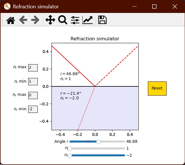
• 3 sliders for $i$, $n_i$ and $n_r$ ;
• 4 text boxes to adjust the range of the sliders for $n_i$ and $n_r$ ;
• 1 button to reset the figure.

Initialization

In this part we simply define the default values of the figure, as well as values that are used to position the interactive elements.

fig,ax = plt.subplots(num="Refraction simulator")
plt.subplots_adjust(bottom=0.25)
plt.title("Refraction simulator")

# Initial value
i = 30      # degrees
n_i = 1     # index of refraction
n_r = 1.5

# Default slider range
n_i_min = 1
n_i_max = 2 
n_r_min = 1
n_r_max = 4

# Slider dimensions
slider_x = .375
slider_y = .05

# Text box dimensions
box_x = .15
box_y = .375
box_height = .05

l_i, l_r, l_rx, r_rad = plot_refraction(fig, ax, i, n_i, n_r)

Compared to the previous figure, the plt.subplots_adjust(bottom=0.25) ensures we have some space below the figure to place our sliders.

Adding the interactive elements

Adding the interactive objects to the figure

This part is a little bit tedious. We have to create an ax object for each interactive object, which will define their position and size. Then, we define the interactive objects themselves on their respective ax objects.

# Sliders for angle and IORs

ax_slider_angle = plt.axes([slider_x, slider_y + .1, .3, .03])
slider_angle = Slider(ax_slider_angle, label="Angle $i$",
                      valmin=0, valmax=90, valinit=i)

ax_slider_n_i = plt.axes([slider_x, slider_y + .05, .3, .03])
slider_n_i = Slider(ax_slider_n_i, label="$n_i$", 
                    valmin=n_i_min, valmax=n_i_max, valinit=n_i)

ax_slider_n_r = plt.axes([slider_x,.05,.3,.03])
slider_n_r = Slider(ax_slider_n_r, label="$n_r$", 
                    valmin=n_r_min, valmax=n_r_max, valinit=n_r)


# Text boxes for the slider range

ax_slider_n_i_max = plt.axes([box_x,box_y+.3,.05,box_height])
box_n_i_max = TextBox(ax_slider_n_i_max, label="$n_i$ max  ",
                      initial = str(n_i_max))

ax_slider_n_i_min = plt.axes([box_x,box_y+.2,.05,box_height])
box_n_i_min = TextBox(ax_slider_n_i_min, label="$n_i$ min  ",
                      initial = str(n_i_min))

ax_slider_n_r_max = plt.axes([box_x,box_y+.1,.05,box_height])
box_n_r_max = TextBox(ax_slider_n_r_max, label="$n_r$ max  ",
                      initial = str(n_r_max))

ax_slider_n_r_min = plt.axes([box_x,box_y,.05,box_height])
box_n_r_min = TextBox(ax_slider_n_r_min, label="$n_r$ min  ",
                      initial = str(n_i_min))


# Reset button

resetax = plt.axes([0.8, .5, 0.1, 0.1])
button = Button(resetax, 'Reset', color='gold', hovercolor='skyblue')

I also added an annotation which displays the angles and refractive indices :

def gen_annot_text(i, r_rad, n_i, n_r):
    r = np.rad2deg(r_rad)
    r = np.round(r,2)
    i = np.round(i,2)
    n_i = np.round(n_i,2)
    n_r = np.round(n_r,2)
    annot_text = f"$i = {i}°$\n$n_i = {n_i}$\n\n\n$r = {r}°$\n$n_r = {n_r}$"
    return annot_text

annot = ax.annotate(gen_annot_text(i, r_rad, n_i, n_r), (-.4, 0),
                    horizontalalignment='left', verticalalignment='center')

The f-strings are very useful for this kind of purpose. You can directly add variable values in strings by putting them inside brackets { }. In this case I also used TeX equation formatting by putting each line between dollar signs $ $.

We’re almost there ! Now we need to add the update functions.

Slider update

Remember when we made the plot_refraction function return three line objects ? It will be useful now.

We have previously defined a slider object. We will now define a update_slider function that will trigger the figure update each time the slider is moved, by using the on_changed method.

The beginning of the update_slider function simply gets the current slider value.

Warning

Using ax.plot will not work ! It will draw a new figure on top of the previous one. This is why we had to export the line data l_i, l_r and l_rx.

After calculating the new values, using the set_data method will update the line objects instead of drawing new ones. It works the same with set_text for the annotation.

def update_slider(val):
    # get current slider value
    i_val = slider_angle.val
    n_i_val = slider_n_i.val
    n_r_val = slider_n_r.val
    
    # calculate new values
    I,R,Rx,r_rad = calc_rays_coords(i_val, n_i_val, n_r_val)
    
    # update lines and annotation
    l_i.set_data(I)
    l_r.set_data(R)
    l_rx.set_data(Rx)
    annot.set_text(gen_annot_text(i_val, r_rad, n_i_val, n_r_val))
    
    return None
    
slider_angle.on_changed(update_slider)
slider_n_i.on_changed(update_slider)
slider_n_r.on_changed(update_slider)

Reset button

This one is easy ! There is a reset method that resets the sliders.

def reset_sliders(event):
    
    slider_angle.reset()
    slider_n_i.reset()
    slider_n_r.reset()

    return None

button.on_clicked(reset_sliders)

Slider range update

Here we use the set_xlim function to adjust the slider ranges. To get the value from the text boxes, we use the text method on the textbox objects. The output is a string, so it has to be converted to a float before using it.

def update_text(text):
    
    slider_n_i.valmin = float(box_n_i_min.text)
    slider_n_i.valmax = float(box_n_i_max.text)
    slider_n_i.ax.set_xlim(slider_n_i.valmin,slider_n_i.valmax)
    
    slider_n_r.valmin = float(box_n_r_min.text)
    slider_n_r.valmax = float(box_n_r_max.text)
    slider_n_r.ax.set_xlim(slider_n_r.valmin,slider_n_r.valmax)

    return None

box_n_i_max.on_submit(update_text)
box_n_i_min.on_submit(update_text)
box_n_r_max.on_submit(update_text)
box_n_r_min.on_submit(update_text)

Results

It’s done ! Now we can visualize refraction, and even play around with exotic refractive indices.