Calculating refraction

Python modules

We will need the following Python modules :

import numpy as np
import matplotlib.pyplot as plt
from matplotlib.patches import Rectangle

Angle calculation

In a refraction problem, you are usually given an incident ray, the IORs of both materials, and you want to calculate the refracted ray angle.

Refraction is described by the Snell-Descartes law : $$ n_i \sin i = n_r \sin r $$ With :

• $i$ the angle of the incident ray (measured from the normal to the interface) ;
• $r$ the angle of the refracted ray ;
• $n_i$ and $n_r$ the respective IORs of the materials.

There will also be a reflected ray of angle $-i$.

Another expression of the Snell’s-Descartes law, better suited to our usage, is : $$ r = \arcsin(\frac{n_i}{n_r}\sin i)$$

Which can be expressed as the following function in Python :

def calc_refraction(i, n_i, n_r):
    i_rad = np.deg2rad(i)
    r_rad = np.asin(n_i/n_r * np.sin(i_rad))
    return r_rad

This function assumes that $i$ is in degrees, but the numpy functions work in radians, hence the need to convert it into $i_{rad} = \frac{\pi}{180}i$.

This function can give a RuntimeWarning in certain situations, but it can be ignored. It corresponds to a total internal reflection, in which no ray is refracted. It’s actually very convenient, because the Matplotlib figure will still work, and the refracted ray will not be displayed.

Ray calculation

We need to plot 3 straight lines, each defined by two points : an incident ray, a refracted ray and a reflected ray. The first point is where they intersect : the origin $(0,0)$. The other extremity of each line can simply be defined by trigonometric functions, in this case they will be placed on a circle of radius 1 :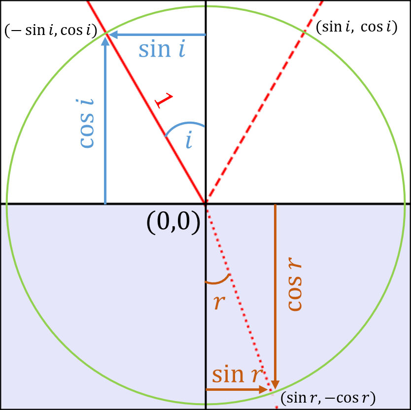

In Python these coordinates are calculated in returned as a [ [x1,x2], [y1,y2] ] list :

def calc_rays_coords(i, n_i, n_r):
    
    i_rad = np.deg2rad(i)
    r_rad = calc_refraction(i, n_i, n_r)

    I = [[-np.sin(i_rad), 0], [np.cos(i_rad), 0]]   # incoming ray
    R = [[0, np.sin(r_rad)], [0, -np.cos(r_rad)]]   # refracted ray
    Rx = [[np.sin(i_rad), 0], [np.cos(i_rad), 0]]   # reflected ray
    
    return I, R, Rx, r_rad

Plotting the figure

The figure is created with the following function :

def plot_refraction(fig, ax, i, n_i, n_r):
    
    I, R, Rx, r_rad = calc_rays_coords(i, n_i, n_r)
    
    ax.set_xlim(-.5,.5)
    ax.set_ylim(-.5,.5)
    ax.set_aspect("equal")  # square figure
    
    l_i, = ax.plot(I[0],I[1],'r',label = "Incoming ray")
    l_r, = ax.plot(R[0],R[1],'r:',label = "Refracted ray")
    l_rx, = ax.plot(Rx[0],Rx[1],'r--',label = "Reflected ray")
    
    ax.plot([-.5, .5],[0, 0],"k")   # boundary between media
    #ax.legend()                    # uncomment to display legend
    ax.add_patch(Rectangle((-0.5, -1), 1, 1, 
                 facecolor="lavender", alpha=1)) # color for second medium
    
    return l_i, l_r, l_rx, r_rad

This function uses the previous one to calculate the coordinates of the lines, then plots a line for each ray. Once again, this function returns variables that will be useful for the interactive plot : the refracted angle in radians r_rad, and the line objects corresponding to the lines that were plotted on the graph l_i, l_r and l_rx. Usually, you might use ax.plot without saving it into a variable, but this will be essential for the next part !

All that’s left to do is use this function :

i = 30      # degrees
n_i = 1     # IOR of air
n_r = 1.5   # IOR of glass

fig = plt.figure("Refraction simulator")
ax = fig.add_subplot(111)

plot_refraction(fig, ax, i, n_i, n_r)

With these values, the result is the following plot :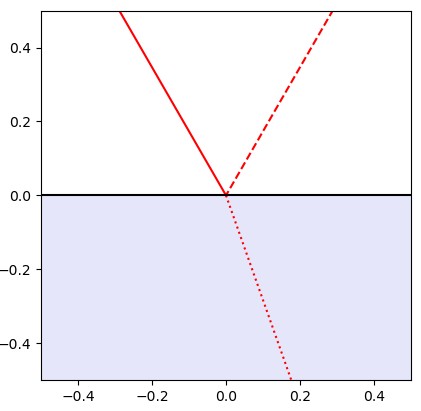

Now we can move on to the interactive part !